Adoption Adjusted Vesting

Introduction of a demand agnostic vesting controller

The Right Token Vesting Terms

What are the right token vesting terms for a new Web3 startup for their fungible token? How do we determine the supply emission rate into a new ecosystem with many unknowns like the actual demand for the token? From experience, working with many founders and looking at the landscape of early crypto startups, it appears there is a lot of insecurity when selecting appropriate token vesting conditions. Founders don’t know if they should introduce a cliff period for some of their early contributors and how long the overall vesting period should be. This article discusses some of the main considerations and introduces a new approach on how to create healthy supply emissions on demand agnostic ecosystems, called Adoption Adjusted Vesting (AAV).

Key Characteristics of AAV

• Demand agnostic algorithmic vesting → the vesting adjusts with respect to measurable ecosystem KPIs instead of inflexible predefined emission tables
• Less token price volatility in the early building phase
• Programmed token price stability or even appreciation
• Variable vesting rates in certain boundaries to ensure compliance with minimum and maximum vesting rate terms
• Early investors contribute to the stability and health of the ecosystem. Simultaneously, they get a more predictable value for their acquired share in tokens
• Individual and even fixed vesting terms for individual stakeholders are still possible
• Vesting weights ensure the right emphasis at the right time for the respective stakeholder group

Vesting State of the Art

Traditionally vesting terms are fixed and will therefore never reflect the best suited solution for a dynamic ecosystem. Web3 ecosystems are fast paced and in many aspects unpredictable. Nevertheless, startups need to decide on and sell vesting terms to their early supporters and investors at a stage where many ecosystem parameters are not well defined.

Fig. 1 and 2 show a stochastic analysis on the vesting cliff and duration of around 50 Web3 startups across a variety of sectors.¹ The cliff in Fig. 1 ranges from 0 to >36 months with mean values around 6 months, depending on the vesting bucket. Vesting durations have a wide range of 0 months up to 9 years with mean values mainly around 18 and 24 months depending on the respective stakeholder. Note that we will publish a more comprehensive stochastic analysis on token launch metrics later. For the purpose of this article the wide range of different vesting terms already shows that there is not a best practice as it highly depends on the considered Web3 sector, the current market conditions, and the respective vesting stakeholder.

Fig. 1: Stochastic evaluation of cliff months of ~100 web3 startups across all sectors

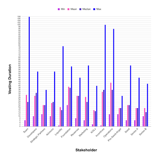Fig. 2: Stochastic evaluation of vesting durations of ~100 web3 startups across all sectors

Fig. 3 reveals another challenge that most of these state-of-the-art vesting regimes produce. In traditional vesting schedules the majority of the supply gets emitted into the ecosystem at the early building phase of the product suite. In other words a lot of supply hits low market demand. This aspect can be simulated by our Quantitative Token Model (QTM) and shows the expected outcome of a dropping token price that only has a chance to recover once enough demand for the token is there through revenue / user upscaling.

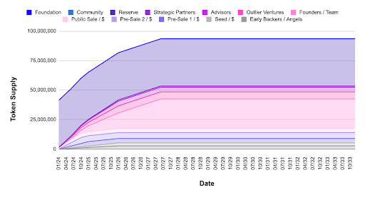Fig. 3: Typical ecosystem development with a full supply release within the first 3 years after TGE and corresponding price drop

Fig. 4 illustrates this price action on an in-market example. In this case the ecosystem is active, but it is still in a building phase and the early investors sell their vested tokens to recoup their initial investment. There is nothing wrong with it per se, but such volatile token prices bring a lot of dissatisfaction to other early investors and potential product adopters.²

What would happen, if the vesting schedule would be extended? Will this necessarily be helpful for the ecosystem and token price stability? The answer is: “It depends.” Longer vesting schedules may not cause such drastic drops in token valuations within the first years and can shift the supply releases to higher market demand after the business building phase moves into the scaling phase. This may result in more sell pressure at later stages and therefore slows down token valuation growth.

Note that very long vesting schedules can lead to supply shocks at token launches and therefore lead to high price spikes that will potentially be sold back down again. “Pump and dump” price action also depends on the actual valuations and liquidity depth, but in any case it is not a good start for a project as many early potential contributors and customers could get hurt.

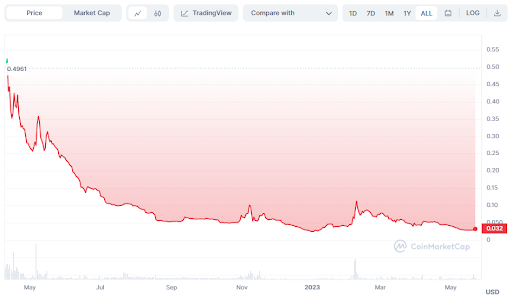Fig. 4: Common price action of young crypto tokens with much selling pressure from vesting parties and too less adoption / demand for the token. Source: coinmarketcap.com

Adoption Adjusted Vesting

The previous section outlined how important the equilibrium between supply release and the actual market demand is for token price stability. In general, too short and also too long vesting schedules can hurt an ecosystem. What can be considered as “too short” or “too long” depends on the individual case and can never be predicted as it depends heavily on the wider market conditions, speculation, and the utility demand for the token.

Therefore an AAV approach can help to solve the dilemma. Milestone vesting heads already in this direction, where certain ecosystem or product milestones need to be reached for a next supply batch to be released. Even though this approach might be helpful in some cases, there are still the big unknowns around the actual numbers and it could potentially introduce transient price spikes through the additional supply release and market manipulation by big market participants around those target dates.

A more flexible and smooth approach is algorithmic token vesting according to certain KPIs. Algorithmic optimization within token ecosystems is not new. Incentive rates for liquidity adoption in DeFi protocols are often determined by controllers that increase the rewards in lower adoption and decrease the rewards in higher adoption phases. In the case of vesting tokens could be issued into the ecosystem depending on TVL, user acquisition / token holder count, revenue thresholds, locking allocations, or the token price itself. Looking at the example of TVL the token vesting rate could be increased in phases of low protocol TVL to have more tokens to incentivise deposits through higher rewards. However, for the sake of simplicity, generality, and scope of this ideating article the token valuation will be considered as an approximation for the protocol adoption. Therefore the token price will be used to algorithmically steer token emission rates into the ecosystem to illustrate the concept.

S	Supply
t	Time
Pl	Implied price
DA	Derivative amplifier
Dy	Average days per year (365.25)
ΔSy, min	Minimum prescribed token issuance per year
ΔSy, max	Maximum prescribed token issuance per year

Eq. 1 is an example on how a supply emission rate could be calculated for the current time step. Note that there are many ways on how a controller for this task could be modeled and displayed. Further views and optimizations are encouraged. Here the supply emission rate for the current time step dS(t)/dt depends on the emission rate of the previous time step dS(t-1)/dt which will be scaled up or down according to an implied price P_l. The higher the penultimate price P(t-2) and the price velocity of the previous time step d/P(t-1)dt multiplied by a derivative amplifier D_A are, the higher the token emission for the next time step. Higher token emissions should then bring the price back down and vice versa. The minimum and maximum prescribed yearly token issuance rates Δ_{Sy, min} and Δ_{Sy, max} ensure that there will always be a minimum amount of tokens released to accomplish full vesting after a maximum set amount of days. Also a maximum token issuance cap is introduced to prevent emitting too many tokens in cases of peak bubble speculation phases.

In any case the best controller design can’t create a stable or even appreciating token price action without demand for the token. However this algorithmic approach can help in supporting a more healthy price action in cases where a threshold minimum demand exists.

In this example the token price has been leveraged as an input signal and as a target implied value for the controller. Note that any input signal could be coupled with any implied parameter (KPI) to optimize for.

Case Study Simulation

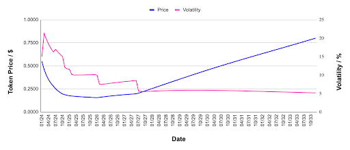
The simulation results in Fig. 5 illustrate how algorithmically controlled token emissions according to Eq. 1 can stabilize the price action for different demand growth scenarios. The top left diagram shows the abstract demand for the token in $-denomination, the top right diagram shows the supply issuance rate per day, the bottom left diagram shows the circulating supply, and the bottom right diagram shows the token price development over the simulation time period.

At the beginning of all scenarios the initial supply release into the ecosystem causes the token price to plummet below the implied price of $0.035. The controller reacts by adjusting the supply release rate to the lower cap, which leads to price appreciation. In the linear demand growth scenario, the implied price can be reached after 2 months and the full supply dilution is accomplished after 27.6 months. The exponential growth scenario is marked by very low initial demand, therefore token release rates stay at the lower cap for 9 months. After reaching the implied price level, token emissions in the exponential growth scenario get ramped up and pass the rates of the other scenarios. Here full supply dilution is reached after 30.8 months. The logistic growth scenario is characterized by the opposite. Since most relative growth happens at the beginning, the controller needs to cap the token emissions at their upper limit. After 6.5 months the token emissions keep up with the demand to bring the price back down to the implied value. It is the fastest supply emission scenario and reaches full dilution after 22.6 months. After full supply dilution the prices in all scenarios start to lift off from the implied value since there are no more external token emissions into the ecosystem that can balance out the increasing demand.

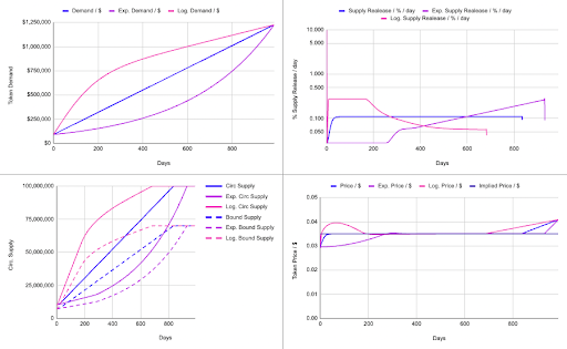Fig. 5: Token demand, daily emission rates, circulating supply, and price for an exemplary ecosystem with adoption adjusted vesting via algorithmic emission controller for different demand scenarios. DA=22

Note that all scenarios assume a constant supply bound ratio of 0.7. This abstract value can be thought of as supply that is not available for sale to meet the demand. In this simulation price is calculated by the demand divided by the available supply, which is 30% of the circulating supply at each time step, respectively.

In this exemplary simulation a constant implied price P_l is assumed. However, it could likewise be a time or other KPI dependent function. E.g. the implied price could simply be rising constantly over time. This would come at the cost of slower vesting. Furthermore the implied price could be steered by a second controller that depends on other ecosystem KPIs, such as the user acquisition or the TVL. These types of more advanced couplings require more in-depth investigation in future works.

The results of the macro simulation in Fig. 5 show the power of a demand agnostic controller for the supply vesting rates. The controller doesn’t know anything about the actual market demand and only takes historical price data into account. Morphing the volatile price action into stabilization comes at the cost of variable vesting terms. The vesting velocity and the corresponding accomplishment date of full supply dilution becomes variable through the controller. With more token demand the vesting is accelerated and vice versa.

The definition of vesting caps, such as given in Eq.1, provides boundaries to ensure that all stakeholders will receive their promised tokens. However, they’d need to agree on the variable vesting rates. Even though this might appear unusual, it might be in favor of initial investors as they contribute to a stabilized ecosystem with appealing and healthy price action and provide more confidence for later investors. Overall these mechanics could therefore create a flywheel that attracts more value to the ecosystem and leads to even faster vesting compared to traditional vesting terms in cases of strong adoption scenarios.

Individual Stakeholder Terms

Now the question regarding individual stakeholder vesting arises. Considering the variable token emissions, there is still uncertainty around the respective share division between each stakeholder at different points in time. Table 1 shows an exemplary scenario of supply allocations and vesting weights for 3 aggregated stakeholder groups. Here the ecosystem incentivisation is prioritized over the team and early investors at the beginning to bootstrap the user and contributor base. At the end of a prescribed period the investors get the higher priority as the ecosystem incentivisation should converge into a circular and sustainable economy instead of being dependent on initial reserves. The team should in any case have the longest vesting period and therefore the least vesting weights as it signals long-term motivation to all external stakeholders.

	Investor	Team	Incentivization
	Supply Allocation / %
	25	20	55
	Vesting Weights / %
Start	15	15	70
End	75	20	5
Table 1: Supply allocations and vesting weights for different aggregated stakeholder groups

Fig. 6 illustrates how the actual vesting rates for the individual stakeholders look like when the vesting weights from Table 1 are applied to the linear growth scenario (blue) of Fig. 5. The incentivisation vesting rate is the highest at the early building stage and declines over time as incentivisation should come out of sustainable sources in the long run. On the other hand the investor vesting rate increases and they reach their full allocation after 600 days. As soon as one aggregated stakeholder group has been fully vested, their share of the overall available vested tokens per time step will be redistributed among the left over stakeholders. This can be observed by the discrete increases in token release rates for the team and incentivisation groups, respectively.

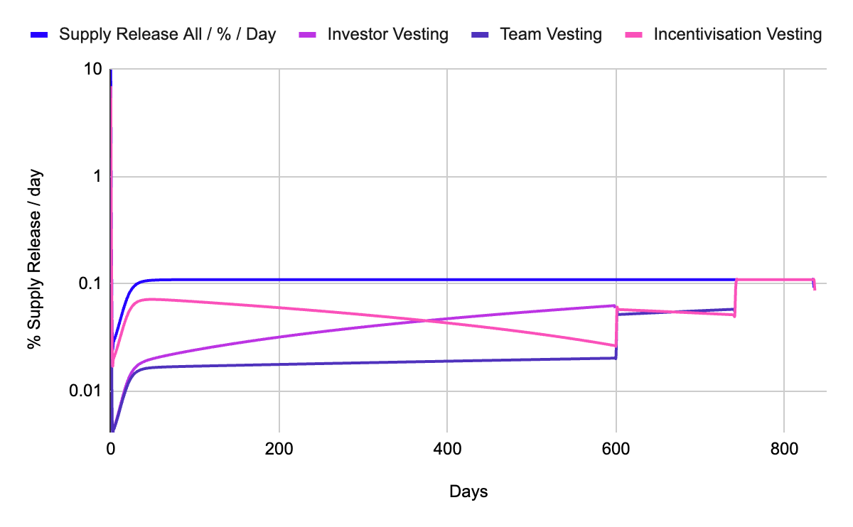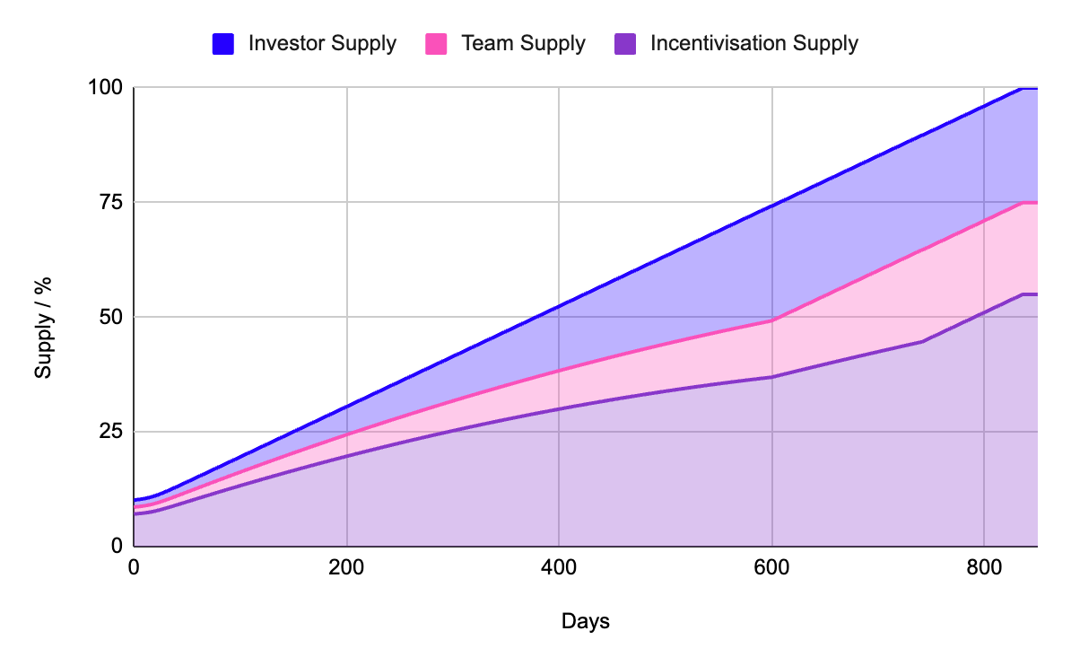Fig. 6: Individual stakeholder shares for demand agnostic AAV via an algorithmic controller w.r.t. vesting weights from Table 1 for the linear growth scenario

Fig. 7 shows the individual stakeholder vesting rates and supply for the exponential and logistic growth scenarios, defined in Fig. 5. Note that there are different time scales on the abscissa according to the varying vesting rates. In any case the vesting weights of the individual groups are respected and all parties receive their allocations eventually.

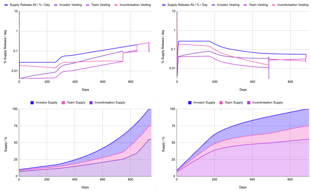Fig. 7: Individual stakeholder shares for demand agnostic AAV via an algorithmic controller w.r.t. vesting weights from Table 1 for the exponential (left) and logistic (right) growth scenarios

These vesting terms are of exemplary nature and depend on the actual fundraising agreements. The approach provides full transparency and flexibility to all ecosystem participants. In cases where certain stakeholders need fixed vesting rates, they still can be incorporated but at the cost of others. E.g. the ecosystem incentivisation vesting could be at fixed rates while the other stakeholders share the leftover variable vesting amounts.

Conclusion

Traditional fixed token emission schedules for an ecosystem will never be able to serve it in the most effective way. In most cases too much supply hits an ecosystem with too little demand in its early building phase and there are many unpredictable aspects that make it impossible to engineer the perfect fixed vesting schedule for all stakeholder groups. This article introduces a demand agnostic adoption adjusting vesting controller that releases token supply according to predefined KPIs. The token emissions are not tied to some set project milestones or key dates, but happen gradually and thereby preventing any transient market manipulations around those key points in time.

In this article the token price has been leveraged as an approximation for the ecosystem adoption and serves as the main input signal for the vesting controller. As soon as the recent token price is above the implied price, the controller increases the token issuance rate and vice versa. Note that implied prices can be variable and even enforce increasing prices at the cost of overall longer vesting periods. The price stabilizing AAV can be compared to algorithmic stable coins, but with one main difference: There is no death spiral instability possible as the vesting rates will always be capped to the upside and to the downside. In high demand phases the token vesting won’t rise infinitely and in low demand periods there will always be tokens vested to ensure the satisfaction of all stakeholder groups.

Early investors might ask themselves what variable vesting will do to their investment. AAV brings flexibility into the full diluted supply allocation target date and therefore adds a layer of uncertainty. On the other hand token prices should tend to more healthy volatility levels and therefore benefit the long-term sustainability of a new ecosystem. Even with slower vesting the tokens will potentially be worth more and therefore compensate for longer waiting periods. Obviously the whole concept of AAV only works for tokens with real demand. Without in-market demand for a token the best controller can’t bring valuations up. In cases of successful ecosystems with appreciating demand for the token, AAV can even lead to accelerated vesting compared to traditional schedules and therefore leverages a good investment choice.

The AAV approach is still a theoretical concept and therefore requires in-market testing. Nevertheless this approach shows a lot of potential for the emergence of more stable and mature token ecosystems in the future.

Outlier Ventures – a strong partner for your Web3 business

Outlier Ventures (OV) empowers crypto start-ups to become successful through holistic expert advisory, networking, and fundraising. Their token economies department provides guidance for NFTs, token design, and token engineering. It leverages powerful tools, such as token design workshops and quantitative token models, to forecast the business idea of Web3 teams or to review and finalize their own token design and model. Applications for OVs’ Base Camp Accelerator for brand new start-up teams or our Ascent program for advanced teams are open. Visit our website for more information: https://outlierventures.io/.

Notes

¹ The underlying database is still in its building phase. It contains data of 239 token launches from 2021 to March 2023 across all sectors. Here only the most recent 50 launches are considered. There will be another article that discusses it in more detail. For the purpose of this article, it just serves as an indication of magnitude for the discussed parameters. Also note that not every startup contains necessarily all displayed vesting buckets.

² Note that the considered time period mainly reflects the recent crypto bear market, which has likewise a significant influence

Acknowledgement

Thanks to Dimitrios Chatzianagnostou, Robert Mullins, Karim Halabi, and Jan Baeriswyl for taking the time to discuss and provide feedback on this new vesting approach.