Introduction
Web3 is a fast moving space with high volatility in user migrations and price charts. Existing Web2 businesses and startups that aim to transition into the Web3 area encounter a new world of complexity, challenges, and opportunities. Once they have decided to embark on this journey, there are many uncertainties and questions that need to be answered. Previous articles discuss the reasons why an initiative might need or want to have a cryptographic token and why quantitative approaches are essential to build a sustainable token business. This report iterates on the quantitative aspect by introducing a generalized Quantitative Token Model (QTM). Instead of explaining the detailed mathematical relationships, it provides a methodological overview along with a case study of a generalized token economy. The QTM is a spreadsheet based tool to model and forecast a majority of known token designs on a higher level where it leverages aggregated stakeholder representation. Even though code-based solutions, such as cadCAD, provide more flexible and sophisticated ways to model the complexity of token ecosystems, the spreadsheet implementation of the QTM has one major benefit: It is accessible to a wider audience and serves a variety of different token business concepts all in one tool.
This document starts with presenting the input and internal structure of the QTM. Afterwards a case study is carried out for a strong and weak user adoption scenario of a fictional Web3 business. Note that the presented token design is not recommended and should not be seen as a benchmark token design for similar businesses. A conclusion at the end wraps up the major findings.
Structure and relevance of the QTM input components
The structure of the QTM consists of 3 main blocks: (1) The ecosystem input section, (2) the utility modules section, and (3) the analysis section. The ecosystem input section is subdivided into the following fundamental subsections:
Basic Token Parameters
- Decision making regarding token supply dynamics / fixation
- Amount of initial token supply
- Launch date of the token (liquidity deployment)
The decision between a dynamic or fixed token supply is fundamental for the whole ecosystem. In the case of dynamic supply the quantitative analysis can be used to adjust the emission for improved token valuation sustainability, while in the fixed supply case it can be used to ensure the project bucket token sustainability. See this article to understand the difference between these two types of sustainability.
Fundraising Module
- Fundraising parties
- Monetary allocations
- Token discounts
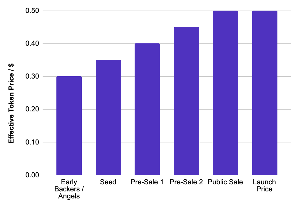
Figure 1 shows the exemplary token prices for different early investor groups. Traditionally more early contributors will receive a cheaper effective token price while they have to commit for longer time vesting schedules. Note that extreme discrepancies between early VC discounted token prices and public sale prices can have a negative impact on future marketing and reputation efforts for the business. Note that not all the different fundraising stages need to be used, the template should be adapted to an individual team’s strategy.
Initial Token Allocations & Vesting Schedules
- Token allocations to initial investor groups, supporting parties, team, protocol buckets, and liquidity
- Individual vesting schedules for each of these entities
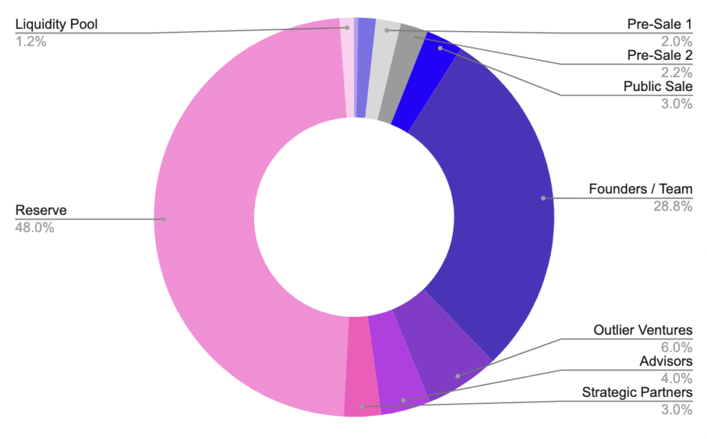
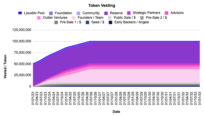
Figures 2 and 3 below indicate some exemplary token allocations and vesting schedules. Note that the given numbers are not optimized, but rather represent historic and experience based allocation magnitudes. Also note that some project buckets are not used in this example. The low share of tokens for liquidity is a problem for many projects if there are not enough token sinks holding the rest of the supply back from being sold into the liquidity pool (LP). This leads often to drastically decreasing token valuations. Performing forecasts with the QTM has the benefit of identifying those sustainability issues before the token has even launched and increases the probability of a supply and price sustainable token circulation.
Liquidity Pool Module
- Token launch price
- Monetary allocation to the LP
- Paired token information
The amount of money that is allocated to the LP is known as liquidity depth and is essential for the price velocity. A deep LP will require more capital to move the price than a LP with less capital. At deployment the LP will consist of the project’s native token and a paired token. The paired one is most often a stable coin or a reputable high market cap token, such as $ETH. In cases where teams can’t afford deep initial liquidity, they have to incentivize other parties to provide it.
User Adoption Module
- Initial user number
- Initial investment per user
- Regular capital inflow per user per month
- Share between product and token buys of user funds
- User behavior in terms of token selling and token utility adoption
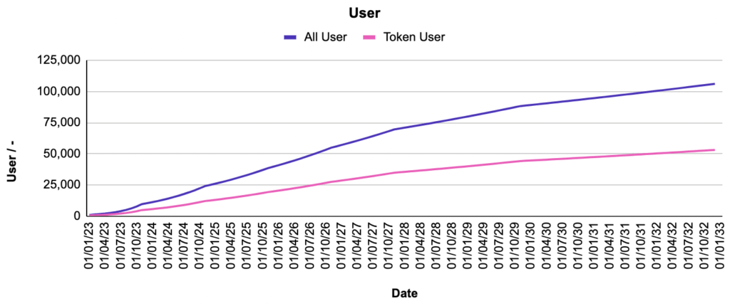
Figure 4 shows an exemplary chart of user growth over the course of 10 years of a Web3 business. This module is essential for the whole ecosystem forecast and based on assumptions regarding the market adoption. The team has to perform market research to estimate the input user growth numbers and the corresponding capital the users will contribute to the ecosystem. The QTM distinguishes further between general users of the whole ecosystem, including off-chain offers and the users that interact with the token. Note that the user adoption must always be treated in different scenarios and can be based on previous similarity market studies.
Business Assumptions
- One time fundraising
- Avg. monthly income streams
- One time investments & expenditures
- Avg. monthly expenditures
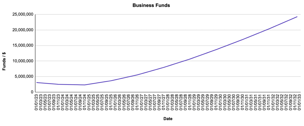
The business assumptions are used to forecast the financial sustainability of the business by balancing the initial raised capital/expenditures and regular income/expenditure streams. Figure 5 shows the business funds growth for an exemplary case. The business funds are equivalent to the equity that is owned by the business, which might be originated by raised investor capital and revenues.
Utility Modules
All previously mentioned aspects are part of the fundamental token ecosystem input section. Another QTM section is dedicated to potential utilities for the token. Note that one can distinguish between different definitions of utility. Instead of “token utility” being exclusively tied to the product interaction, in this article “token utility” refers to a broader spectrum on which a token can be used. This includes liquidity provision, staking, payments, burning, and holding of the token. In the QTM the utilities are built in a modular way, so that project teams can not only activate or deactivate certain utilities, but also set their assumed weighting with respect to token allocations and specific parameters for each individual one. Figure 6 shows the 5 generalized utilities that are implemented in the current QTM version (1.8).
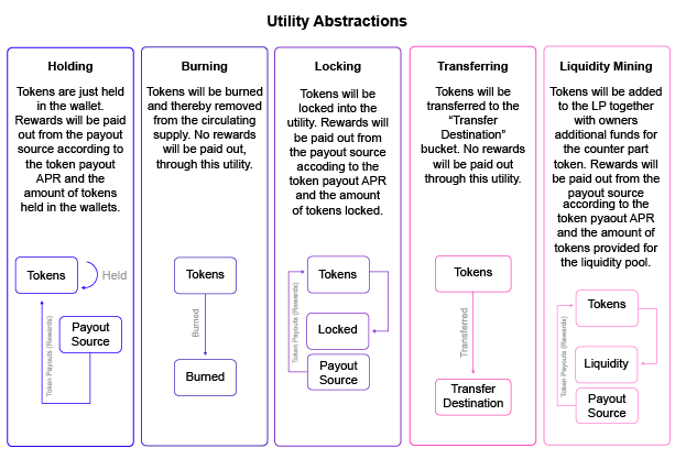
Holding
The “Holding” utility is for projects that want to pay out token rewards to wallets that hold the token to incentivize further holding.
Locking
The “Locking” utility can be used as representation for staking or play to earn concepts, where users lock their tokens into a smart contract to receive more tokens as rewards.
Liquidity Mining
The “Liquidity Mining” utility is created to incentivize other parties to provide liquidity through additional token rewards.
Burning
The “Burning” utility has to be used to account for token burnings.
Transfer
The “Transfer” utility is used whenever tokens will be transferred from token holders back to project buckets. E.g. this can be used for a shop where users can buy items in exchange for the token or to pay for services / fees.
Another optional utility mechanic not mentioned in the above list is an off-chain point system that can be used to have more control over value emission to the stakeholders. It leverages off-chain points that can be reused for the products or can be converted into the token and thereby being sold or used for the other utilities. Optionally users that stake the token can get a multiplier on their token issuance rate. Figure 7 illustrates the point issuance with and without multiplier along with the resulting token emissions through the conversion from points to tokens.
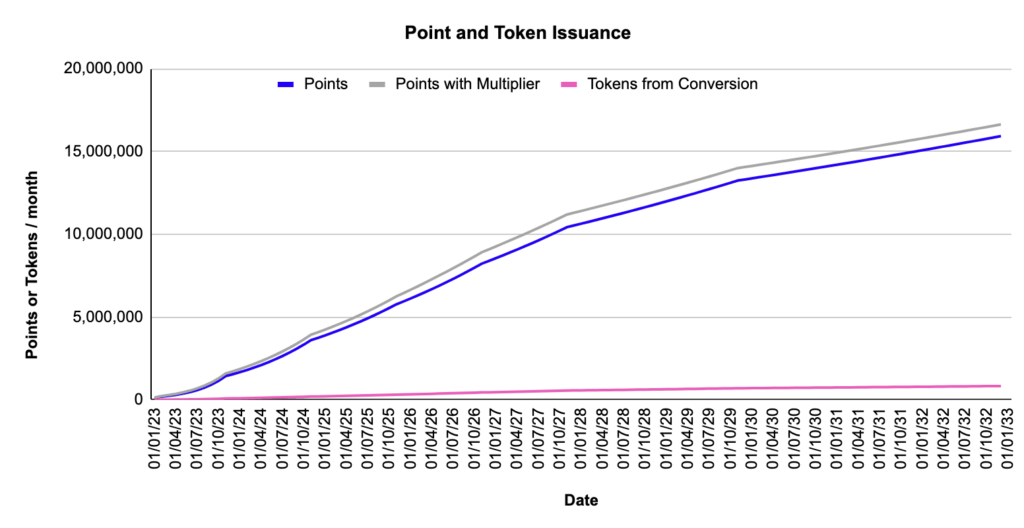
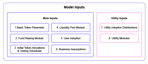
Figure 8 shows an overview of all previously mentioned input modules for the QTM. Note that all of the subsections need to be fed with the most accurate data available, since the quality of the output depends mainly on the quality of the input data and assumptions made in the QTM.
QTM Structure
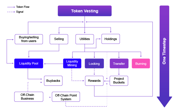
The QTM’s abstracted structure is shown in Figure 9, where the rough processing order for one timestep is from the top to the bottom. The QTM is a time-domain model with a fixed timestep of one month and a simulation range of 10 years. Each timestep starts with the token distribution from the vesting schedules of the different early investor groups. These “free” tokens will be categorized into three meta buckets. One is used for selling tokens into the LP. The liquidity is implemented as an Automated Market Maker (AMM) LP with the widely known constant product relationship. Another meta bucket for the vested tokens is used to distribute the tokens to all enabled utilities, specified in the utility modules input section. The last meta bucket is for all tokens freely held by the users and other ecosystem participants. Note that “Holding” can also be defined as an utility, such as outlined before. The distribution shares for all meta bucket categories and the individual utilities have to be set by the designer using the QTM. Every timestep users can join or leave the ecosystem with their capital. This is represented by varying user growth, capital spending for the product or buying the token, selling the token, and utility allocations or removals. Rewards are defined within the individual utilities and will be paid out to stakeholders, while the transfer utility can be used for a refilling of the project buckets. Note that the off-chain business can also buyback tokens to further sustain the project token buckets and issue off-chain points as another layer of value feedback. The model doesn’t leverage Monte Carlo simulations since it already represents the arithmetic mean of all inputs and outputs. Furthermore, it doesn’t include any Markov decision making trees options since all decisions are preset by the designer through average token allocation shares that are constant for the whole course of the simulation. Hence aggregated representative stakeholders are assumed. Note that transient events can be implemented through manual manipulation of the input tables. These simplifications are not sufficient for comprehensive and realistic ecosystem analyses, but they are made as a tradeoff to mitigate complexity for the model to increase accessibility for a wider audience while serving as many different Web3 concepts as possible through its generalized modular framework. Even though predictions won’t be accurate they can provide a first quantitative approximation.
Case Study
Introduction
Two of the main goals for the ecosystem modeling token engineer is to maintain token value and supply sustainability. Choosing a dynamic token design will mitigate the token supply sustainability issue, since tokens can be minted infinitely, but this mechanic has to be counterbalanced through burning, buybacks, and/or increasing demand for the token to maintain value sustainability. On the other hand a fixed supply token can be attractive for investors since they know that they can own a fixed share of the represented business without getting diluted through potential token inflation. A fixed supply of tokens requires token sustainability, since there must always be enough tokens left in the reserves to pay out rewards for the stakeholders of different utilities. In any case the token has to capture and accrue value to be attractive for investors.
The presented case study considers a token design with moderate token emissions for two different user adoption scenarios and discusses the implications of main ecosystem parameters.
Case Study – Base Setup
The following case study illustrates the difference between a strong user adoption and a lower user adoption for a Web3 business that sells a product or service in exchange for their token. The product requires a subscription fee of $3 worth of token per month per user. Also users can stake their tokens or participate in a liquidity mining program to receive token rewards. The business has to sell the received tokens from the subscription fees to cover their costs and to make a profit. The initial supply is set to 100,000,000 tokens, the early investor groups, token distribution and vesting is defined as in the example inputs given in Figures 1 to 3. It is assumed that the protocol raises a total amount of $3.9m before the token generation event (TGE). The token has a launch price of $0.50 and 15 % of the raised capital is used to purchase the paired token for the DEX LP. This results in the initial valuations given in the following table:
| LP | $1,170,000 |
| MC | $25,957,500 |
| FDV MC | $50,000,000 |
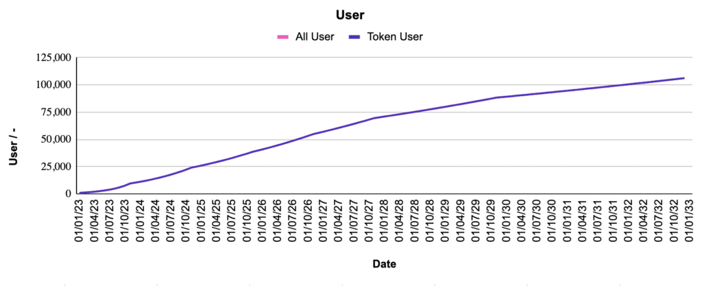
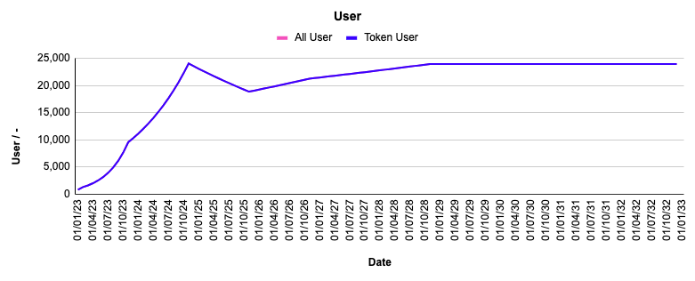
The user adoption is shown in Figure 10, where the amount of token users equals the amount of overall business users, since they need the token to participate for every provided offer. In the case study an additional scenario with one negative growth year and growth stagnation is assumed, represented by the curve in Figure 11. The strong user growth curve ends with 106,167 users and the weak growth scenario ends with 25,412 users after the simulation period of 10 years.
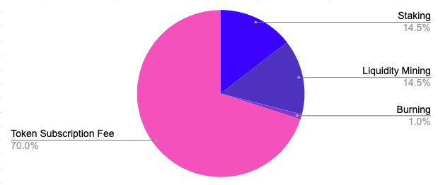
Since the main utility for the token is either spending it for the product subscription or letting it produce yields within the staking or the liquidity mining program, it is assumed that 75 % of the free supply is used for utilities, 20 % will be sold and 5 % will be held in the wallets. Besides this 3 % of the utility allocations will be removed every month as an average assumption. The utility allocations are assumed to be distributed as shown in Figure 12 for every timestep. The rewards for staking and liquidity mining are 15 % and 30 % APR respectively and are generated through a minting function. The majority token utility allocation of 70 % is assumed to be used to pay for the product subscription. 1 % of all utility allocated tokens will be burned per month. Those tokens are subtracted from the product subscription.
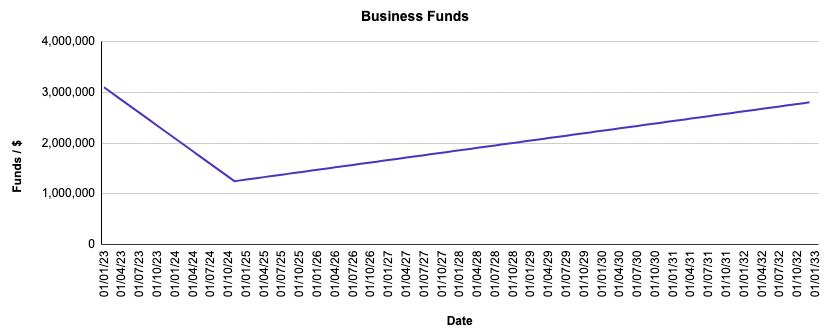
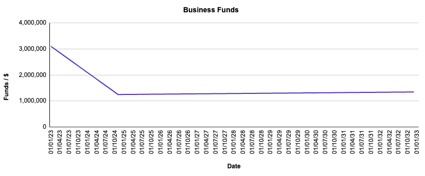
For the business a one-time investment of $50k is assumed to cover initial debts. Furthermore regular costs of $84k per month are assumed for the salaries, software licenses, and other expenditures. The income for the business is set to a constant amount of $100k per month and gained from token sales starting two years after the TGE. The resulting funds development without consideration of business token holdings is shown in Figure 13.
Since the income is a $-denominated fixed value, it is not affected by the two different user growth curve scenarios. However, the different user growth assumptions affect other case study specific metrics, discussed in the following sections.
Scenario I: Strong User Adoption
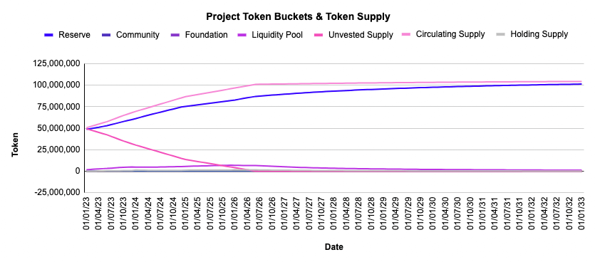
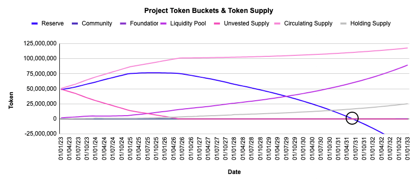
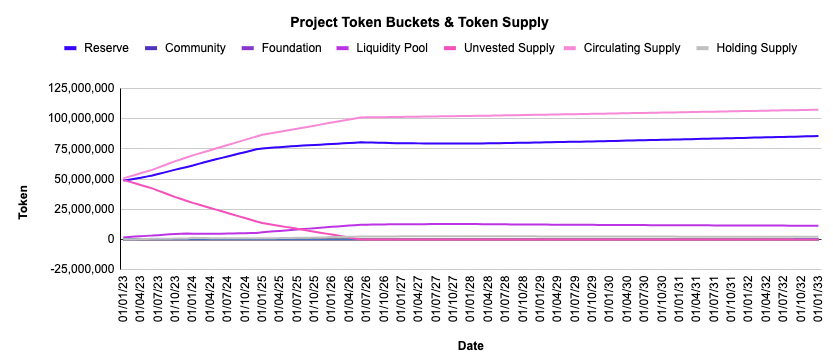
The strong user growth scenario is based on the numbers given in Figure 10. The project buckets and the supply numbers of the token are the first important metrics to analyze. Figure 14 shows their development over the course of the simulation. The initial investor vesting ends 3.5 years after the TGE. The circulating supply increases through this vesting period to around 100m tokens and continues to rise slightly due to the token minting for payouts to staking and liquidity mining participants. The token reserves also increase over time, since they are filled from the customers transferring their tokens to pay for the main product subscription.
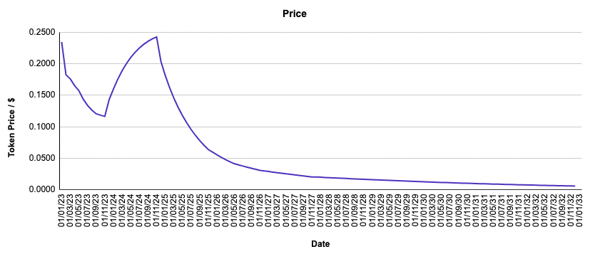
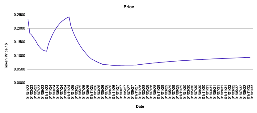
The strong user growth creates demand for the token so that its price starts to appreciate after the bottom of $0.12 per token is reached after one year. The initial decrease of the token price is caused by the sell pressure from the vested tokens from initial investor groups combined with the comparatively low user count of just 9,537 at the end of the first year. One big advantage of the QTM simulation tool is that input parameters can be changed without much effort. In this case it is of interest to examine the effect of another vesting schedule. E.g. changing it to double vesting time for all early investors would result in an initial token price drop to just $0.19.
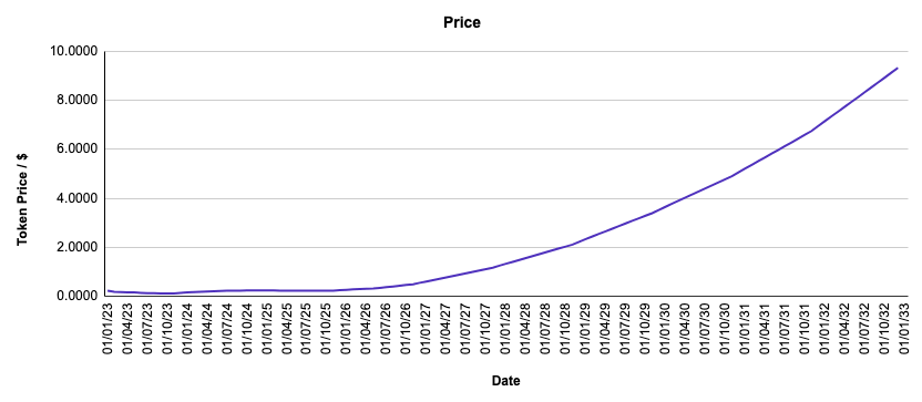
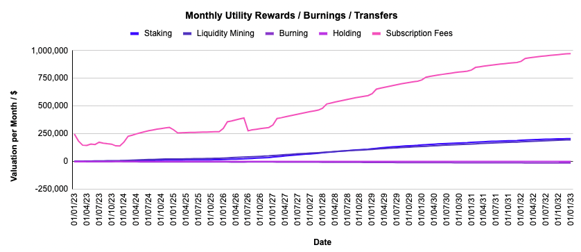
Figure 16 shows the $-denominated value flows from and to the different utilities respectively. They show the expected healthy growth coinciding with the user growth. At the end of the simulation period, the transferred amount of tokens from the users approaches $1m, while around $400k worth of tokens are issued to stakers and liquidity miners as reward and $14k worth of tokens are burned per month.
Scenario II: Weak User Adoption
The weak user growth scenario is based on the numbers given in Figure 11. The token supplies in Figure 17 reveal that the reserve bucket will run out of tokens after around 8 years, since too few users counterbalance the constant token selling from the business. Note that even the dynamic setup of the token can’t sustain the strong sell pressure in terms of token supply.
Similarly the token price experiences a massive drop in the negative growth year, which coincides with the start of the regular massive token sales from the business. Overall the applied business setup is not sustainable in terms of the token valuation and the supply for this low user adoption. The QTM can be leveraged to find settings that might change this unsustainable situation into a sustainable one.
Reducing the monthly token sales from $100k to $85k worth of tokens is already enough to reach a sustainable token valuation and token price. These numbers will not lead to strong business fund growth, but let the business sustain, such as indicated in Figure 19.
Figures 20 and 21 show the corresponding token supply and valuation curves for this survival mode scenario. Now the reserves supply is sustainable over the simulation period and the price starts rising again after the negative growth year. Note that external market psychological factors are not accounted for in these simulations, which means that the appearance of the price chart doesn’t affect the behavior of the users and investors in the model. This simplified assumption is a limitation of the QTM.
Conclusion
The case study shows some capabilities of the QTM, where fundamental token business aspects are evaluated within seconds after parameter definition. This specific analysis revealed the impact of different user adoption scenarios and showcased how small changes in the base parameters can cause the difference between a sustainable and an unsustainable Web3 business. The QTM is a powerful and accessible tool with a clean UI to perform high level forecasts for many different kinds of token ecosystems. It is built in a modular structure so that token designers and engineers can turn on and off whatever functionality they want. The QTM leverages customizable token supply designs, fund raisings, token allocations, vesting schedules, liquidity pool designs, user adoption scenarios, (static) user behaviors, business assumptions, buyback strategies and on- and off-chain utilities. The tool is programmed in a spreadsheet so that everyone can use it without any coding knowledge and simulates each given setup within a few seconds. It is the ideal tool for new Web3 businesses and existing businesses to create a first quantitative iteration for their token design while allocating low time resources for setting the simulation up.
Outlook
Even though this model is suitable for most of the Web3 businesses, some concepts are too complex to be represented by a generalized tool. Therefore we are building more sophisticated tools in the background that will leverage state-of-the-art high performance token engineering approaches and combine them with new on-chain data-driven decision making processes.
Outlier Ventures – a strong partner for your web3 business
Outlier Ventures empowers crypto start-ups to become successful through holistic expert advisory, networking, and fundraising. Their token economies department provides guidance for NFTs, token design, and token engineering. It leverages powerful tools, such as token design workshops and quantitative token models, to forecast the business idea of Web3 teams or to review and finalize their own token design and model. Applications for OVs’ Base Camp Accelerator for brand new start-up teams or our Ascent program for advanced teams are open. Visit our website for more information: https://outlierventures.io/.
Dr. Achim Struve joined Outlier Ventures as token engineer, where he developed the first generalized data-driven Quantitative Token Model (QTM) with focus on accessibility for founders. Achim also performs in-depth on-chain analyses via own data scraping and processing algorithms to extract behavioural insights of already launched projects. Before joining Outlier, Achim completed his doctoral thesis (summa cum laude), where he gained his expertise about complex systems modelling, optimization, and data analyses.